This is a very nice collection of the USGS R training curriculum, and materials that correspond to specific workshops. The current courses are Introduction to R, Introduction to USGS R Packages, and R Package Development.
Introduction to R Languages can be found here:
https://owi.usgs.gov/R/training-curriculum/intro-curriculum/.
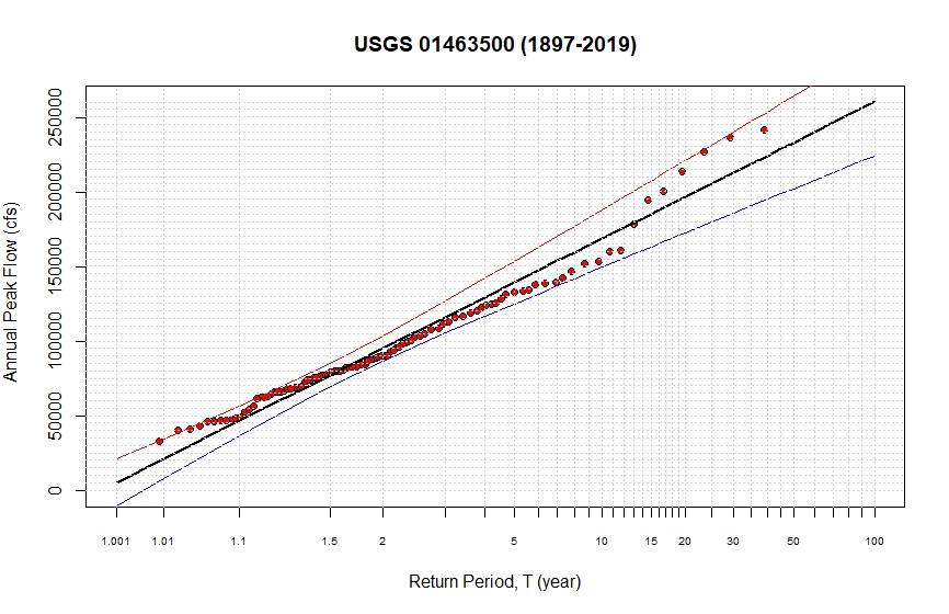
I also developed a sample R program to analyze the flood recurrence interval based on annual peak discharge (cfs), and Log-Pearson Type III distribution at USGS 01463500 Delaware River at Trenton NJ:
### Removing all previously generated datasets and plots
cat("\014")
rm(list = ls())
dev.off()
### STEP 2
### Loading two specific packages into Program
library(dataRetrieval)
library(xts)
### STEP 3
### Get the Peak Annual Discharge at USGS Delaware River at Trenton, NJ
mysite<-'01463500'
annualpeak<-readNWISpeak(mysite)
### STEP 4
### Perform Flood Frequency Analysis
Q_peak = as.numeric(annualpeak$peak_va)
Q <- na.exclude(Q_peak)
graphlab = "(1897-2019)"
#Generate plotting positions
n = length(Q)
r = n + 1 - rank(Q) # highest Q has rank r = 1
T = (n + 1)/r
# Set up x-axis tick positions and labels
Ttick = c(1.001,1.01,1.1,1.5,2,3,4,5,6,7,8,9,10,11,12,13,14,15,16,17,18,19,20,25,30,35,40,45,50,60,70,80,90,100)
xtlab = c(1.001,1.01,1.1,1.5,2,NA,NA,5,NA,NA,NA,NA,10,NA,NA,NA,NA,15,NA,NA,NA,NA,20,NA,30,NA,NA,NA,50,NA,NA,NA,NA,100)
y = -log(-log(1 - 1/T))
ytick = -log(-log(1 - 1/Ttick))
xmin = min(min(y),min(ytick))
xmax = max(ytick)
# Fit a line by method of moments, along with 95% confidence intervals
KTtick = -(sqrt(6)/pi)*(0.5772 + log(log(Ttick/(Ttick-1))))
QTtick = mean(Q) + KTtick*sd(Q)
nQ = length(Q)
se = (sd(Q)*sqrt((1+1.14*KTtick + 1.1*KTtick^2)))/sqrt(nQ)
LB = QTtick - qt(0.975, nQ - 1)*se
UB = QTtick + qt(0.975, nQ - 1)*se
max = max(UB)
Qmax = max(QTtick)
# Plot peak flow series with Gumbel axis
plot(y, Q,
ylab = expression( "Annual Peak Flow (cfs)" ) ,
xaxt = "n", xlab = "Return Period, T (year)",
ylim = c(0, Qmax),
xlim = c(xmin, xmax),
pch = 21, bg = "red",
main = paste( "USGS 01463500",graphlab )
)
par(cex = 0.65)
axis(1, at = ytick, labels = as.character(xtlab))
# Add fitted line and confidence limits
lines(ytick, QTtick, col = "black", lty=1, lwd=2)
lines(ytick, LB, col = "blue", lty = 1, lwd=1.5)
lines(ytick, UB, col = "red", lty = 1, lwd=1.5)
# Draw grid lines
abline(v = ytick, lty = 3, col="light gray")
abline(h = seq(500, floor(Qmax), 5000), lty = 3,col="light gray")
par(cex = 1)
### STEP 5
# Also show regression equations for Q~T
model <- lm(QTtick~ytick)
paste('Q =', coef(model)[[2]], '* ln(T)', '+', coef(model)[[1]])
paste('T =', 'EXP ( (Q - ', coef(model)[[1]], ') / ', coef(model)[[2]], ')')